If we want to know which values are duplicated in a column, we do the following
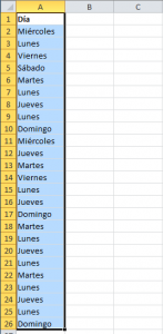
First you must select the data range to which the conditional formatting will be applied:
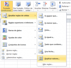
Then you must go to the tab Home and in the group Styles click on Conditional format and then display the menu Highlight cell rules and choose the option Duplicate values.
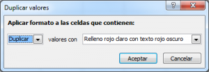
The dialog box will be displayed Duplicate Values.
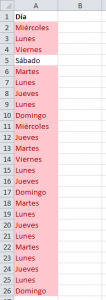
Leave the default options and click OK. All the values are highlighted except Saturday because it is the only one in the entire list that does not repeat itself:


No Comment